Linear model optimal design

Getting started

Optimal designs for linear models are calculated using the R6-class lm_design. When initializing a design object with lm_design$new(), the minimal required inputs are a (discrete) candidate design grid and a one-sided linear model formula:

library(cvxoptdes)

## 3 factors w/ 5, 5 and 3 levels
data <- expand.grid(
  x1 = -2:2,
  x2 = -2:2,
  x3 = -1:1
)

design <- lm_design$new(
  formula = ~(x1 + x2 + x3)^2 + I(x1^2) + I(x2^2) + I(x3^2),   ## full quadratic model
  data = data    ## design points
)

design$data
#>    x1 x2 x3
#> 1  -2 -2 -1
#> 2  -1 -2 -1
#> 3   0 -2 -1
#> 4   1 -2 -1
#> 5   2 -2 -1
#> 6  -2 -1 -1
#> 7  -1 -1 -1
#> 8   0 -1 -1
#> 9   1 -1 -1
#> 10  2 -1 -1
....

After initializing the linear model and design grid, use the $optimize() method to calculate an approximate optimal design:

(design_weights <- design$optimize(criterion = "D")) |> round(2)
#>  [1] 0.06 0.00 0.03 0.00 0.06 0.00 0.00 0.00 0.00 0.00 0.03 0.00 0.00 0.00 0.03 0.00 0.00 0.00 0.00 0.00 0.06 0.00 0.03 0.00 0.06 0.03 0.00 0.00 0.00
#> [30] 0.03 0.00 0.00 0.00 0.00 0.00 0.00 0.00 0.06 0.00 0.00 0.00 0.00 0.00 0.00 0.00 0.03 0.00 0.00 0.00 0.03 0.06 0.00 0.03 0.00 0.06 0.00 0.00 0.00
#> [59] 0.00 0.00 0.03 0.00 0.00 0.00 0.03 0.00 0.00 0.00 0.00 0.00 0.06 0.00 0.03 0.00 0.06
#> attr(,"criterion")
#> attr(,"criterion")$crit.value
#> [1] 1.897913
#> 
#> attr(,"criterion")$crit
#> [1] "D"

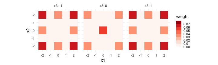
The $optimize() method returns the weights assigned to each design point in design$data, as well as the optimized value of the selected design criterion, which upper bounds the criterion value for any integer optimal design.

Use the $round() method to round the approximate optimal design to an exact (integer) design with a given number of observations. If method = "optimal", a number of repeated point-exchange procedures are executed to find an optimal exact design:

## integer design w/ 13 design points
(exact_design <- design$round(m = 13, method = "optimal", seed = 1))
#>  [1] 1 0 0 0 1 0 0 0 0 0 1 0 0 0 0 0 0 0 0 0 0 0 1 0 1 0 0 1 0 0 0 0 0 0 0 0 0 0 0 1 0 0 0 0 0 1 0 0 0 0 1 0 0 0 1 0 0 0 0 0 0 0 1 0 0 0 0 0 0 0 1 0 0
#> [74] 0 1
#> attr(,"criterion")
#> attr(,"criterion")$crit
#> [1] "D"
#> 
#> attr(,"criterion")$crit.value
#> [1] 1.84352
#> 
#> attr(,"criterion")$crit.rel.eff
#> [1] 0.9713408

Since the point-exchange algorithm is initialized from (a rounded version of) the approximate optimal design, the required number of repeated runs of the point-exchange algorithm (n_repeats) can generally be kept low. 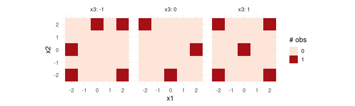The $round() method returns an integer design vector of the same length as design$data, the value of the design criterion and the relative efficiency with respect to the approximate optimal design. As the number of design points (m) in the exact design grows, the relative efficiency converges to 1. The design points in the integer design vector can be obtained by subsetting the design$data grid, or by using the dedicated $subset() method:

design$subset(replicates = exact_design)
#>    x1 x2 x3
#> 1  -2 -2 -1
#> 5   2 -2 -1
#> 11 -2  0 -1
#> 23  0  2 -1
#> 25  2  2 -1
#> 28  0 -2  0
#> 40  2  0  0
#> 46 -2  2  0
#> 51 -2 -2  1
#> 55  2 -2  1
#> 63  0  0  1
#> 71 -2  2  1
#> 75  2  2  1

The lm_design object can be reused to compute optimal designs for other design criteria, or to evaluate other properties of a given design. For instance, the variance-covariance matrix of the linear model parameter estimates, or the correlation matrix of the columns of the design matrix:

design$vcov(design_weights = exact_design, sigma2 = 1) |> round(3)
#>             (Intercept)     x1     x2     x3 I(x1^2) I(x2^2) I(x3^2)  x1:x2  x1:x3  x2:x3
#> (Intercept)       0.722  0.002 -0.002  0.005  -0.070  -0.070  -0.279  0.012 -0.024  0.024
#> x1                0.002  0.025  0.000  0.000  -0.001   0.000   0.000  0.000 -0.001  0.003
#> x2               -0.002  0.000  0.025  0.000   0.000   0.001   0.000  0.000  0.003 -0.001
#> x3                0.005  0.000  0.000  0.101   0.000   0.000  -0.006  0.003 -0.001  0.001
#> I(x1^2)          -0.070 -0.001  0.000  0.000   0.030  -0.003  -0.014  0.000  0.000 -0.008
#> I(x2^2)          -0.070  0.000  0.001  0.000  -0.003   0.030  -0.014  0.000  0.008  0.000
#> I(x3^2)          -0.279  0.000  0.000 -0.006  -0.014  -0.014   0.474 -0.015  0.000  0.000
#> x1:x2             0.012  0.000  0.000  0.003   0.000   0.000  -0.015  0.009 -0.003  0.003
#> x1:x3            -0.024 -0.001  0.003 -0.001   0.000   0.008   0.000 -0.003  0.035 -0.005
#> x2:x3             0.024  0.003 -0.001  0.001  -0.008   0.000   0.000  0.003 -0.005  0.035

design$corr(design_weights = exact_design) |> round(3)
#>             x1     x2     x3 I(x1^2) I(x2^2) I(x3^2)  x1:x2  x1:x3  x2:x3
#> x1       1.000  0.000  0.000   0.000   0.000   0.000  0.000  0.000 -0.112
#> x2       0.000  1.000  0.000   0.000   0.000   0.000  0.000 -0.112  0.000
#> x3       0.000  0.000  1.000   0.000   0.000   0.000 -0.112  0.000  0.000
#> I(x1^2)  0.000  0.000  0.000   1.000   0.133   0.133  0.000  0.000  0.233
#> I(x2^2)  0.000  0.000  0.000   0.133   1.000   0.133  0.000 -0.233  0.000
#> I(x3^2)  0.000  0.000  0.000   0.133   0.133   1.000  0.233  0.000  0.000
#> x1:x2    0.000  0.000 -0.112   0.000   0.000   0.233  1.000  0.125 -0.125
#> x1:x3    0.000 -0.112  0.000   0.000  -0.233   0.000  0.125  1.000  0.125
#> x2:x3   -0.112  0.000  0.000   0.233   0.000   0.000 -0.125  0.125  1.000

The above example covers the main methods to calculate an optimal design with cvxoptdes. The following sections provide additional details on the available optimization objectives and rounding procedures implemented in cvxoptdes and how to use them.

Approximate optimal design

By default, the following optimization problem is solved by the $optimize() method of an R6-object of class lm_design:

\boldsymbol{w}^* = \arg \max_{\boldsymbol{w} \in \Delta^n} \Phi(M(\boldsymbol{w}\ |\ \boldsymbol{X}, \boldsymbol{v}) + \lambda I) - \alpha \cdot \boldsymbol{c}' \boldsymbol{w}

Here,

$\boldsymbol{w} = (w_1,\ldots, w_n)'$ is the vector of (continuous) design weights, with $w_i \in [0, 1]$ and $\sum_{i = 1}^n w_i = 1$ .
$\boldsymbol{c} = (c_1,\ldots, c_n)'$ is a cost assigned to each design weight scaled by the (global) penalty parameter $\alpha$ .
$M(\boldsymbol{w}\ |\ \boldsymbol{X}, \boldsymbol{v})$ is the information matrix of the linear model depending on the weights $\boldsymbol{w}$ and the $(n \times p)$ design matrix $\boldsymbol{X}$ , and possibly a vector of fixed user weights $\boldsymbol{v} = (v_1, \ldots, v_n)'$ in the case of weighted linear regression.
$\Phi(M)$ is the design optimality criterion as a (scalar) function of the information matrix $M$ .

Given the linear model formula, the $(p \times p)$ information matrix, conditional on the error variance $\sigma_e^2$ , is given by:

M(\boldsymbol{w}\ |\ \boldsymbol{X}, \boldsymbol{v}) \ = \ \frac{1}{\sigma_e^2} \sum_{i = 1}^n w_i v_i \boldsymbol{x}_i \boldsymbol{x}_i'

where $\boldsymbol{x}_i$ is the i-th design point or the i-th row in the design matrix $\boldsymbol{X}$ constructed with model.matrix. If $\lambda > 0$ in the optimization problem, a ridge term is added to the diagonal of $M$ resulting in the information matrix of a ridge linear regression model. This is particularly useful when $n < p$ to ensure a non-singular information matrix for the evaluation of the optimality criterion $\Phi(M)$ .

When calling the $optimize() method, the penalized optimization problem is solved efficiently as a convex second-order cone program (SOCP) using the open-source Splitting Cone Solver (SCS). For D-optimal designs, the SOCP is formulated using spectral cones introduced in (Cederberg and Boyd 2025). For I-, A-, and G-optimal designs, the SOCP formulations of (Sagnol and Harman 2015) are used. At the moment of writing, the $optimize() method supports the following optimality criteria:

D-optimality : Maximize the volume (determinant) of the information matrix $M$ , or equivalently minimize the volume of the confidence ellipsoid of the parameter estimates. For D-optimality, the logarithm of the D-criterion is used for optimization:

\Phi(M) = \log\left(\det(M)^{1/p}\right)

design$optimize(criterion = "D") |> round(2)
#>  [1] 0.06 0.00 0.03 0.00 0.06 0.00 0.00 0.00 0.00 0.00 0.03 0.00 0.00 0.00 0.03 0.00 0.00 0.00 0.00 0.00 0.06 0.00 0.03 0.00 0.06 0.03 0.00 0.00 0.00
#> [30] 0.03 0.00 0.00 0.00 0.00 0.00 0.00 0.00 0.06 0.00 0.00 0.00 0.00 0.00 0.00 0.00 0.03 0.00 0.00 0.00 0.03 0.06 0.00 0.03 0.00 0.06 0.00 0.00 0.00
#> [59] 0.00 0.00 0.03 0.00 0.00 0.00 0.03 0.00 0.00 0.00 0.00 0.00 0.06 0.00 0.03 0.00 0.06
#> attr(,"criterion")
#> attr(,"criterion")$crit.value
#> [1] 1.897913
#> 
#> attr(,"criterion")$crit
#> [1] "D"

A-optimality: Maximize the inverse trace of the inverse information $M^{-1}$ , or equivalently minimize the average variance of the parameter estimates:

\Phi(M) \ = \ \text{Tr}(M^{-1})^{-1}

design$optimize(criterion = "A") |> round(2)
#>  [1] 0.04 0.00 0.01 0.00 0.04 0.00 0.00 0.00 0.00 0.00 0.01 0.00 0.09 0.00 0.01 0.00 0.00 0.00 0.00 0.00 0.04 0.00 0.01 0.00 0.04 0.02 0.00 0.04 0.00
#> [30] 0.02 0.00 0.00 0.00 0.00 0.00 0.04 0.00 0.19 0.00 0.04 0.00 0.00 0.00 0.00 0.00 0.02 0.00 0.04 0.00 0.02 0.04 0.00 0.01 0.00 0.04 0.00 0.00 0.00
#> [59] 0.00 0.00 0.01 0.00 0.09 0.00 0.01 0.00 0.00 0.00 0.00 0.00 0.04 0.00 0.01 0.00 0.04
#> attr(,"criterion")
#> attr(,"criterion")$crit.value
#> [1] 0.07981045
#> 
#> attr(,"criterion")$crit
#> [1] "A"

I-optimality: Maximize the inverse of the average prediction variance across the design space, (equivalently minimize the average prediction variance):

\Phi(M) = \left(\frac{1}{n} \sum_{i = 1}^n \boldsymbol{x}_i' M^{-1} \boldsymbol{x}_i\right)^{-1}

design$optimize(criterion = "I") |> round(2)
#>  [1] 0.05 0.00 0.04 0.00 0.05 0.00 0.00 0.00 0.00 0.00 0.04 0.00 0.04 0.00 0.04 0.00 0.00 0.00 0.00 0.00 0.05 0.00 0.04 0.00 0.05 0.03 0.00 0.02 0.00
#> [30] 0.03 0.00 0.00 0.00 0.00 0.00 0.02 0.00 0.07 0.00 0.02 0.00 0.00 0.00 0.00 0.00 0.03 0.00 0.02 0.00 0.03 0.05 0.00 0.04 0.00 0.05 0.00 0.00 0.00
#> [59] 0.00 0.00 0.04 0.00 0.04 0.00 0.04 0.00 0.00 0.00 0.00 0.00 0.05 0.00 0.04 0.00 0.05
#> attr(,"criterion")
#> attr(,"criterion")$crit.value
#> [1] 0.1213055
#> 
#> attr(,"criterion")$crit
#> [1] "I"

G-optimality: Maximize the inverse of the maximum prediction variance across the design space, (equivalently minimize the maximum prediction variance):

\Phi(M) = \left(\max_{\boldsymbol{x}_i} \boldsymbol{x}_i' M^{-1} \boldsymbol{x}_i\right)^{-1}

design$optimize(criterion = "G") |> round(2)
#>  [1] 0.06 0.00 0.03 0.00 0.06 0.00 0.00 0.00 0.00 0.00 0.03 0.00 0.00 0.00 0.03 0.00 0.00 0.00 0.00 0.00 0.06 0.00 0.03 0.00 0.06 0.03 0.00 0.00 0.00
#> [30] 0.03 0.00 0.00 0.00 0.00 0.00 0.00 0.00 0.06 0.00 0.00 0.00 0.00 0.00 0.00 0.00 0.03 0.00 0.00 0.00 0.03 0.06 0.00 0.03 0.00 0.06 0.00 0.00 0.00
#> [59] 0.00 0.00 0.03 0.00 0.00 0.00 0.03 0.00 0.00 0.00 0.00 0.00 0.06 0.00 0.03 0.00 0.06
#> attr(,"criterion")
#> attr(,"criterion")$crit.value
#> [1] 0.09999999
#> 
#> attr(,"criterion")$crit
#> [1] "G"

alias-optimality: Maximize one minus the average absolute cosine similarity (also uncentered correlation or normalized dot product) between the columns of the design matrix:

\Phi(\boldsymbol{w}, \boldsymbol{X}) \ = \ 1 - \frac{2}{p(p - 1)} \sum_{1 \leq q < r \leq p} \left| \frac{M_{qr}}{\sqrt{M_{qq}} \sqrt{M_{rr}}} \right|

If the weighted design columns are all centered in the sense that $\sum_i {w_i} x_{iq} = 0$ for $q = 1,\ldots,p$ , this criterion is equivalent to minimizing the average absolute correlation between the weighted design columns.

design$optimize(criterion = "alias", scs_control = list(eps_rel = 1e-3)) |> round(2)
#>  [1] 0.12 0.00 0.01 0.00 0.12 0.00 0.00 0.00 0.00 0.00 0.01 0.00 0.00 0.00 0.01 0.00 0.00 0.00 0.00 0.00 0.12 0.00 0.01 0.00 0.12 0.00 0.00 0.00 0.00
#> [30] 0.00 0.00 0.00 0.00 0.00 0.00 0.00 0.00 0.00 0.00 0.00 0.00 0.00 0.00 0.00 0.00 0.00 0.00 0.00 0.00 0.00 0.12 0.00 0.01 0.00 0.12 0.00 0.00 0.00
#> [59] 0.00 0.00 0.01 0.00 0.00 0.00 0.01 0.00 0.00 0.00 0.00 0.00 0.12 0.00 0.01 0.00 0.12
#> attr(,"criterion")
#> attr(,"criterion")$crit.value
#> [1] 0.8678501
#> 
#> attr(,"criterion")$crit
#> [1] "alias"

Exact optimal design

Optimal rounding

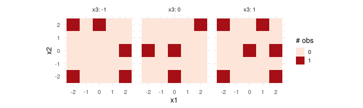
As demonstrated in the initial example, the $round() method is used to round an approximate (optimal) design to an exact integer design with a given number of observations. The default rounding method is "optimal" rounding, which executes a number (n_repeats) of repeated Fedorov point-exchange procedures (Fedorov 1972) starting from randomly sampled versions of the distribution of approximate design weights, or from efficiently rounded designs (Pukelsheim and Rieder 1992) if the size of the exact design is sufficiently large. The optimality criterion is recycled from the "criterion" attribute in the design weights vector (design$design_weights) populated by $optimize(), but can be overridden by passing a new criterion to $round() itself. Instead of starting the rounding procedure from a rounded version of the approximate design in design$design_weights, it is also possible to provide a custom weight vector via the design_weights argument or to round from a random initial design by setting design_weights = FALSE.

(exact_design <- design$round(m = 15, method = "optimal", criterion = "I", design_weights = design_weights, n_repeats = 100, seed = 1))
#>  [1] 1 0 0 0 1 0 0 0 0 0 0 0 0 0 1 0 0 0 0 0 1 0 1 0 0 0 0 1 0 0 0 0 0 0 0 1 0 1 0 0 0 0 0 0 0 0 0 0 0 1 1 0 0 0 1 0 0 0 0 0 0 0 1 0 1 0 0 0 0 0 1 0 0
#> [74] 1 0
#> attr(,"criterion")
#> attr(,"criterion")$crit
#> [1] "I"
#> 
#> attr(,"criterion")$crit.value
#> [1] 0.1137218
#> 
#> attr(,"criterion")$crit.rel.eff
#> [1] NA

Efficient rounding

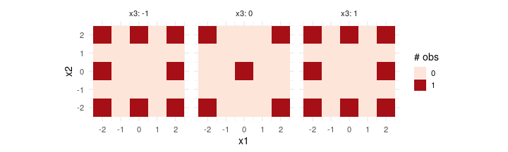
The "efficient" rounding method is included for completeness only, as this is used for (efficient) initial rounding of the approximate design weights to serve as a starting point for the point-exchange algorithm in "optimal" rounding. The "efficient" rounding method requires the number of requested design points m to be larger than (or equal to) the size of the support of the approximate design.

(exact_design <- design$round(m = 21, method = "efficient", criterion = "D", design_weights = design_weights * (design_weights > 0.01), seed = 1))
#>  [1] 1 0 1 0 1 0 0 0 0 0 1 0 0 0 1 0 0 0 0 0 1 0 1 0 1 1 0 0 0 1 0 0 0 0 0 0 0 1 0 0 0 0 0 0 0 1 0 0 0 1 1 0 1 0 1 0 0 0 0 0 1 0 0 0 1 0 0 0 0 0 1 0 1
#> [74] 0 1
#> attr(,"criterion")
#> attr(,"criterion")$crit
#> [1] "D"
#> 
#> attr(,"criterion")$crit.value
#> [1] 1.866278
#> 
#> attr(,"criterion")$crit.rel.eff
#> [1] 0.9833318

Distance-based rounding

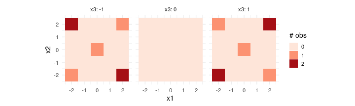
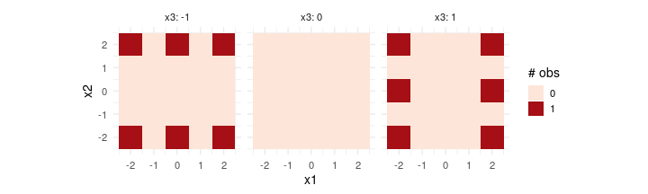
The "dist-sum" and "dist-min" rounding methods maximize the distances between rows of the candidate design matrix, or equivalently, maximize exploration of the design space. The rounded designs are calculated using point-exchange methods that are independent of the selected design criterion. The "dist-sum" rounding procedure maximizes the total pairwise (Euclidean) distance between design matrix rows of the integer design. The "dist-min" rounding procedure maximizes the minimum pairwise (Euclidean) distance between design matrix rows. These distance-based methods are primarily of interest for small rounded designs, where the number of requested design points m is (much) smaller than the total number of candidate design points, i.e. $m \ll n$ .

(dist1_design <- design$round(m = 14, method = "dist-sum", seed = 1))
#>  [1] 1 0 0 0 2 0 0 0 0 0 0 0 1 0 0 0 0 0 0 0 2 0 0 0 1 0 0 0 0 0 0 0 0 0 0 0 0 0 0 0 0 0 0 0 0 0 0 0 0 0 2 0 0 0 1 0 0 0 0 0 0 0 1 0 0 0 0 0 0 0 1 0 0
#> [74] 0 2
#> attr(,"criterion")
#> attr(,"criterion")$crit
#> [1] "dist-sum"
#> 
#> attr(,"criterion")$crit.value
#> [1] 729.7219
#> 
#> attr(,"criterion")$crit.rel.eff
#> [1] NA

(dist2_design <- design$round(m = 12, method = "dist-min", seed = 1))
#>  [1] 1 0 1 0 1 0 0 0 0 0 0 0 0 0 0 0 0 0 0 0 1 0 1 0 1 0 0 0 0 0 0 0 0 0 0 0 0 0 0 0 0 0 0 0 0 0 0 0 0 0 1 0 0 0 1 0 0 0 0 0 1 0 0 0 1 0 0 0 0 0 1 0 0
#> [74] 0 1
#> attr(,"criterion")
#> attr(,"criterion")$crit
#> [1] "dist-min"
#> 
#> attr(,"criterion")$crit.value
#> [1] 5.656854
#> 
#> attr(,"criterion")$crit.rel.eff
#> [1] NA

Parallel evaluation

The repeated point-exchange algorithms run by the $round() method can be executed in parallel using mirai. The number and type of parallel background R processes is configured by the user before calling $round() with mirai::daemons(). If daemon connections are available, $round() automatically runs in asynchronous mode using the configured daemons:

library(mirai)

daemons(n = parallel::detectCores() / 2, seed = 1)     ## use half the number of available cores

design$round(m = 100, method = "optimal", n_repeats = 1000)

daemons(0)   ## close daemons

Remark: the implemented exchange algorithms depend heavily on low-level BLAS and LAPACK routines. If the BLAS/LAPACK routines already execute on multiple threads, this may interfere with the asynchronous evaluation of mirai. In this case, it is recommended to restrict BLAS/LAPACK to a single thread by setting the environment variables OPENBLAS_NUM_THREADS, MKL_NUM_THREADS or OMP_NUM_THREADS, depending on the BLAS library being used. In addition, there is a small overhead in populating the environments of the background R processes to prepare the evaluations. In rare cases, this leads to a higher computation time than sequential evaluation in the main R process, especially when n_repeats is small or the execute time of a single repeat of the exchange algorithm is almost negligible.

Penalized optimal design

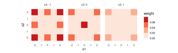
By penalized or weighted optimal design, we refer to optimization of the design criterion subject to a user-defined cost penalty or weight assigned to each candidate design point. Heterogeneous weights or costs can be included in the design optimization problem in two ways; either through the weight vector $\boldsymbol{v} = (v_1,\ldots,v_n)'$ or through the cost vector $\boldsymbol{c} = (c_1,\ldots,c_n)'$ . The weights $\boldsymbol{v}$ are incorporated as multiplicative terms on the level of the information matrix, whereas the costs $\boldsymbol{c}$ are penalizing the optimality criterion value using an additive penalty term. Both options have intuitive interpretations; a heterogeneous weight vector $\boldsymbol{v}$ produces the optimal design of a weighted linear regression model. For a non-zero cost vector $\boldsymbol{c}$ , the optimization problem above is the dual form (with Lagrange multiplier $\alpha$ ) of the cost-constrained design optimization problem:

\boldsymbol{w}^* = \arg \max_{\boldsymbol{w} \in \Delta^n} \Phi(M(\boldsymbol{w}\ |\ \boldsymbol{X}, \boldsymbol{v}) + \lambda I), \quad \quad \text{subject to} \quad \boldsymbol{c}'\boldsymbol{w} \leq B

for some design budget $B$ . An advantage of using the multiplicative weights $\boldsymbol{v}$ is that the weighted optimal design is invariant under scaling of $\boldsymbol{v}$ . This is not the case when scaling the penalty parameter $\alpha$ or the costs $\boldsymbol{c}$ , which change the contribution of the additive penalty term in the optimization problem.

To add costs $\boldsymbol{c} = (c_1,\ldots,c_n)'$ to the optimization problem, we can either re-initialize the design object with lm_design$new() (including a cost argument) or update the existing object:

## assign c = 1 if x3 = 1, and c = 0 otherwise
design$update(
  cost = ~pmax(x3, 0),
  alpha = 1
)

The $update() method accepts the same arguments as lm_design$new(), which means that the linear model (formula) or the candidate design grid (data) can also be updated if needed. Here, we assigned a cost $c_i = 1$ to all design points with x3 = 1 and a cost $c_i = 0$ otherwise. This could be a scenario where the design points with level x3 = 1 are more expensive or time-consuming to evaluate. The penalty parameter $\alpha$ is set to $\alpha = 1$ . Increasing $\alpha$ increases the importance of the assigned costs relative to the optimality criterion $\Phi(M)$ .

design$optimize(criterion = "D") |> round(2)
#>  [1] 0.07 0.00 0.06 0.00 0.07 0.00 0.00 0.00 0.00 0.00 0.06 0.00 0.00 0.00 0.06 0.00 0.00 0.00 0.00 0.00 0.07 0.00 0.06 0.00 0.07 0.05 0.00 0.01 0.00
#> [30] 0.05 0.00 0.00 0.00 0.00 0.00 0.01 0.00 0.08 0.00 0.01 0.00 0.00 0.00 0.00 0.00 0.05 0.00 0.01 0.00 0.05 0.04 0.00 0.00 0.00 0.04 0.00 0.00 0.00
#> [59] 0.00 0.00 0.00 0.00 0.00 0.00 0.00 0.00 0.00 0.00 0.00 0.00 0.04 0.00 0.00 0.00 0.04
#> attr(,"criterion")
#> attr(,"criterion")$crit.value
#> [1] 1.488574
#> 
#> attr(,"criterion")$crit
#> [1] "D"

Remark: The returned criterion value is the value of the penalized design criterion including the penalty term $\alpha \cdot \boldsymbol{c}' \boldsymbol{w}^*$ . To evaluate the design criterion excluding the cost penalty term, use the $crit() method with alpha = FALSE. By default, the criterion value is returned for the approximate design present in the $design_weights field:

design$crit(criterion = "D", alpha = FALSE)
#> [1] 1.722761

Similarly, weights $\boldsymbol{v} = (v_1, \ldots, v_n)'$ can be added to the optimization problem by updating the existing object using the weights argument:

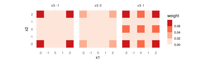
## assign v = 1 if x3 = 1, and v = 0.1 otherwise
design$update(
  weights = ~pmax(x3, 0.1),
  cost = NULL
)

Unlike the additive costs $\boldsymbol{c}$ , the multiplicative weights $\boldsymbol{v}$ are required to be positive. Note also that the influence of the weights on the optimized design is opposite to that of the costs $\boldsymbol{c}$ : design points with a high cost $c_i$ are discouraged in the optimal design, whereas design points with a high weight $v_i$ are preferred.

design$optimize(criterion = "D") |> round(2)
#>  [1] 0.07 0.00 0.00 0.00 0.07 0.00 0.00 0.00 0.00 0.00 0.00 0.00 0.00 0.00 0.00 0.00 0.00 0.00 0.00 0.00 0.07 0.00 0.00 0.00 0.07 0.03 0.00 0.00 0.00
#> [30] 0.03 0.00 0.00 0.00 0.00 0.00 0.00 0.00 0.00 0.00 0.00 0.00 0.00 0.00 0.00 0.00 0.03 0.00 0.00 0.00 0.03 0.08 0.00 0.05 0.00 0.08 0.00 0.00 0.00
#> [59] 0.00 0.00 0.05 0.00 0.06 0.00 0.05 0.00 0.00 0.00 0.00 0.00 0.08 0.00 0.05 0.00 0.08
#> attr(,"criterion")
#> attr(,"criterion")$crit.value
#> [1] 0.6481402
#> 
#> attr(,"criterion")$crit
#> [1] "D"

Penalized design rounding

The costs and weights present in the $cost and $weights fields are automatically passed down to the $round() method when "optimal" rounding is used. For "efficient" rounding, the costs/weights are not used explicitly, but are taken into account implicitly because this procedure rounds to an integer design that is close to the penalized approximate design. For "dist-sum" and "dist-min" rounding, the costs and/or weights are not taken into account and the rounded designs are the same with or without assigned costs and/or weights.

## optimal rounding w/ weights
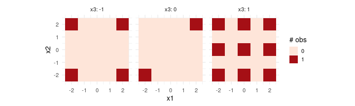
(exact_design <- design$round(m = 15, method = "optimal", seed = 1))
#>  [1] 1 0 0 0 1 0 0 0 0 0 0 0 0 0 0 0 0 0 0 0 1 0 0 0 1 1 0 0 0 0 0 0 0 0 0 0 0 0 0 0 0 0 0 0 0 0 0 0 0 1 1 0 1 0 1 0 0 0 0 0 1 0 1 0 1 0 0 0 0 0 1 0 1
#> [74] 0 1
#> attr(,"criterion")
#> attr(,"criterion")$crit
#> [1] "D"
#> 
#> attr(,"criterion")$crit.value
#> [1] 0.6355939
#> 
#> attr(,"criterion")$crit.rel.eff
#> [1] 0.9806426

Stratified optimal design

The formulation of the approximate optimal design problem as a convex second-order cone program allows for straightforward extension by extra convex (cone) constraints. One relevant (linear) equality constraint is that of a stratified optimal design. Consider a partitioning of the candidate design grid into individual (disjoint) strata $\mathcal{X}_1,\ldots,\mathcal{X}_S$ , then we solve the optimal design problem subject to the constraint that each stratum is represented with a given proportion $p_1,\ldots,p_S$ ( $\sum_s p_s = 1$ ):

\begin{aligned} \boldsymbol{w}^* \ = \ & \arg \max_{\boldsymbol{w} \in \Delta^n} \Phi(M(\boldsymbol{w}\ |\ \boldsymbol{X}, \boldsymbol{v}) + \lambda I) - \alpha \cdot \boldsymbol{c}'\boldsymbol{w}, \\ & \text{subject to } \sum_{\{i\ :\ \boldsymbol{x}_i \in \mathcal{X}_s\}} w_i = p_s, \quad \text{for } s = 1,\ldots,S \end{aligned}

To include stratification constraints in the optimal design problem, the $stratify() method is used. The partitioning into individual strata can be passed as a single factor variable or a one-sided formula containing multiple factors. In the second case, the strata are defined by the unique levels obtained from the interaction() of all factors in the formula.

## drop weights term
design$update(weights = NULL)

## add stratification constraints
design$stratify(
  strata = ~x3,
  proportions = c(1/4, 1/2, 1/4)
)

design$strata
#> $strata
#>  [1] -1 -1 -1 -1 -1 -1 -1 -1 -1 -1 -1 -1 -1 -1 -1 -1 -1 -1 -1 -1 -1 -1 -1 -1 -1 0  0  0  0  0  0  0  0  0  0  0  0  0  0  0  0  0  0  0  0  0  0  0 
#> [49] 0  0  1  1  1  1  1  1  1  1  1  1  1  1  1  1  1  1  1  1  1  1  1  1  1  1  1 
#> Levels: -1 0 1
#> 
#> $proportions
#> [1] 0.25 0.50 0.25

## stratified optimal design
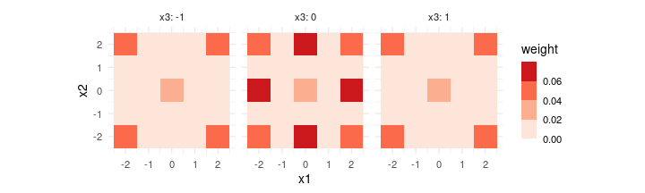
design$optimize(criterion = "D") |> round(2)
#>  [1] 0.05 0.00 0.00 0.00 0.05 0.00 0.00 0.00 0.00 0.00 0.00 0.00 0.02 0.00 0.00 0.00 0.00 0.00 0.00 0.00 0.05 0.00 0.00 0.00 0.05 0.05 0.00 0.06 0.00
#> [30] 0.05 0.00 0.00 0.00 0.00 0.00 0.06 0.00 0.03 0.00 0.07 0.00 0.00 0.00 0.00 0.00 0.05 0.00 0.07 0.00 0.05 0.05 0.00 0.00 0.00 0.05 0.00 0.00 0.00
#> [59] 0.00 0.00 0.00 0.00 0.02 0.00 0.00 0.00 0.00 0.00 0.00 0.00 0.05 0.00 0.00 0.00 0.05
#> attr(,"criterion")
#> attr(,"criterion")$crit.value
#> [1] 1.739444
#> 
#> attr(,"criterion")$crit
#> [1] "D"

## verify stratification
tapply(design$design_weights, design$data$x3, sum)
#>   -1    0    1 
#> 0.25 0.50 0.25

Remark: if the proportions argument in $stratify() is left unspecified, equal weight proportions are assigned to each stratum.

This type of stratification only defines feasibility constraints on the allocation of the design weights. The linear model error structure and information matrix are not changed and should not be confused with the construction of blocked designs, where the block effects are included in the model as nuisance random or fixed effects. See vignette("nlm_lme_design") for the calculation of optimal blocked designs in the context of a (random intercept) linear mixed model.

Stratified design rounding

Similar to rounding of penalized approximate designs, if stratification constraints are present in the $strata field, these are passed down to the $round() method when "optimal" rounding is used. The same is true for "dist-sum" and "dist-min" rounding. For "efficient" rounding, stratification constraints are not enforced explicitly. Note that for integer designs, the stratification constraints can only be satisfied exactly if the strata proportions multiplied by the number of requested design points (m) are all integer.

## optimal rounding w/ stratification
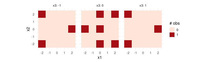
(exact_design <- design$round(m = 12, method = "optimal", seed = 1))
#>  [1] 1 0 0 0 0 0 0 0 0 0 0 0 0 0 1 0 0 0 0 0 1 0 0 0 0 0 0 1 0 1 0 0 0 0 0 1 0 1 0 0 0 0 0 0 0 0 0 1 0 1 1 0 0 0 0 0 0 0 0 0 0 0 0 0 1 0 0 0 0 0 1 0 0
#> [74] 0 0
#> attr(,"criterion")
#> attr(,"criterion")$crit
#> [1] "D"
#> 
#> attr(,"criterion")$crit.value
#> [1] 1.58603
#> 
#> attr(,"criterion")$crit.rel.eff
#> [1] 0.911803
#> 
#> attr(,"strata")
#> -1  0  1 
#>  3  6  3

## drop stratification
design$stratify(strata = NULL)

Design orthogonality constraints

The alias-optimality criterion minimizes the absolute cosine similarity between columns of the design matrix $\boldsymbol{X}$ subject to the design weights $\boldsymbol{w} = (w_1,\ldots,w_n)'$ . Instead of minimizing the cosine similarity, it is also possible to add explicit constraints on the absolute cosine similarities, which are representable as (convex) rotated second-order cone inequalities. For design columns $q$ and $r$ , and a given constraint value $\rho_{qr} \in [0, 1]$ , we can include the following constraint in the design optimization problem:

\left| \frac{\langle \boldsymbol{w} \boldsymbol{x}_{.q}, \boldsymbol{x}_{.r} \rangle}{\Vert \sqrt{\boldsymbol{w}} \boldsymbol{x}_{.q} \Vert \Vert \sqrt{\boldsymbol{w}} \boldsymbol{x}_{.r} \Vert} \right| \ \leq \ \rho_{qr}

To illustrate with an example, it is often desirable for the main effects columns (x1, x2, x3) to be orthogonal to all other design columns to ensure identifiability of the main effects parameters. Orthogonality constraints are specified using the orthogonal argument in lm_design$new() or $update() in the form of a three-part formula, e.g. x1 + x2 + x3 ~ . ~ 0. The first part (x1 + x2 + x3) defines all design columns $\boldsymbol{x}_{.q}$ passed as first argument in the orthogonality constraint using linear model formula notation. The second part (.) defines all design columns $\boldsymbol{x}_{.r}$ passed as second argument in the orthogonality constraint using linear model formula notation. The third part is optional and specifies the constraint value $\rho_{qr}$ for the set of selected design columns. If only a two-part formula is provided, $\rho_{qr}$ is set to zero. A list of formulas can be passed to the orthogonal argument to stack different constraints for different subsets of design columns. To verify that all orthogonality constraints are parsed as expected, the $orthogonal field can be inspected, which returns the $(p \times p)$ constraint matrix $(\rho_{qr})_{q,r}$ :

## orthogonal main effects wrt all other columns
design$update(
  orthogonal = x1 + x2 + x3 ~ . ~ 0
)

design$orthogonal
#>             (Intercept)  x1  x2  x3 I(x1^2) I(x2^2) I(x3^2) x1:x2 x1:x3 x2:x3
#> (Intercept)         Inf   0   0   0     Inf     Inf     Inf   Inf   Inf   Inf
#> x1                    0 Inf   0   0       0       0       0     0     0     0
#> x2                    0   0 Inf   0       0       0       0     0     0     0
#> x3                    0   0   0 Inf       0       0       0     0     0     0
#> I(x1^2)             Inf   0   0   0     Inf     Inf     Inf   Inf   Inf   Inf
#> I(x2^2)             Inf   0   0   0     Inf     Inf     Inf   Inf   Inf   Inf
#> I(x3^2)             Inf   0   0   0     Inf     Inf     Inf   Inf   Inf   Inf
#> x1:x2               Inf   0   0   0     Inf     Inf     Inf   Inf   Inf   Inf
#> x1:x3               Inf   0   0   0     Inf     Inf     Inf   Inf   Inf   Inf
#> x2:x3               Inf   0   0   0     Inf     Inf     Inf   Inf   Inf   Inf

## optimize design w/ orthogonality constraints
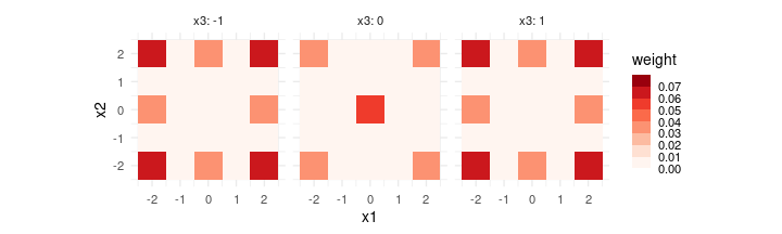
design$optimize(criterion = "D") |> round(2)
#>  [1] 0.06 0.00 0.03 0.00 0.07 0.00 0.00 0.00 0.00 0.00 0.03 0.00 0.01 0.00 0.03 0.00 0.00 0.00 0.00 0.00 0.07 0.00 0.03 0.00 0.07 0.03 0.00 0.00 0.00
#> [30] 0.03 0.00 0.00 0.00 0.00 0.00 0.01 0.00 0.05 0.00 0.01 0.00 0.00 0.00 0.00 0.00 0.03 0.00 0.01 0.00 0.03 0.07 0.00 0.03 0.00 0.07 0.00 0.00 0.00
#> [59] 0.00 0.00 0.03 0.00 0.01 0.00 0.03 0.00 0.00 0.00 0.00 0.00 0.07 0.00 0.03 0.00 0.07
#> attr(,"criterion")
#> attr(,"criterion")$crit.value
#> [1] 1.897913
#> 
#> attr(,"criterion")$crit
#> [1] "D"

Sparse optimal design

The optimized approximate design is in fact identical to an unconstrained D-optimal design, as the optimal solution remains feasible also with the added orthogonality constraints. More interesting is enforcing the orthogonality constraints on a smaller (or sparser) set of support points. Penalties that promote sparsity of the design weight vector $\boldsymbol{w} = (w_1,\ldots,w_n)'$ are generally not convex. For this reason, a sequential convex approximation procedure is implemented, substituting (concave) sparseness penalties by linearized (convex) costs on the design weights.

The sequential convex approximation procedure is available through the $sparsify() method, which runs several iterations of $optimize(), each iteration updating the cost term $\alpha \cdot \boldsymbol{c}' \boldsymbol{w}$ based on the selected (sparsity promoting) reweighting function. Ideally, the maximum number of reweighting iterations is large enough for the weight vector to converge to a stable solution.

## set sparseness penalty
design$update(alpha = 0.75)

## iterative reweighting using entropy-based penalties
design$sparsify(max_iter = 5, criterion = "D", reweight_fun = "entropy") |> round(2)
#>  [1] 0.10 0.00 0.01 0.00 0.10 0.00 0.00 0.00 0.00 0.00 0.01 0.00 0.00 0.00 0.01 0.00 0.00 0.00 0.00 0.00 0.10 0.00 0.01 0.00 0.10 0.01 0.00 0.00 0.00
#> [30] 0.01 0.00 0.00 0.00 0.00 0.00 0.00 0.00 0.12 0.00 0.00 0.00 0.00 0.00 0.00 0.00 0.01 0.00 0.00 0.00 0.01 0.10 0.00 0.01 0.00 0.10 0.00 0.00 0.00
#> [59] 0.00 0.00 0.01 0.00 0.00 0.00 0.01 0.00 0.00 0.00 0.00 0.00 0.10 0.00 0.01 0.00 0.10
#> attr(,"criterion")
#> attr(,"criterion")$crit
#> [1] "D"
#> 
#> attr(,"criterion")$crit.value
#> [1] 1.593979

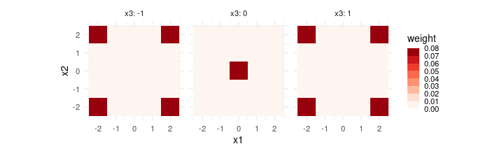
## verify correlations
design$corr() |> round(3)
#>         x1 x2 x3 I(x1^2) I(x2^2) I(x3^2) x1:x2 x1:x3 x2:x3
#> x1       1  0  0   0.000   0.000   0.000     0     0     0
#> x2       0  1  0   0.000   0.000   0.000     0     0     0
#> x3       0  0  1   0.000   0.000   0.000     0     0     0
#> I(x1^2)  0  0  0   1.000   0.757   0.757     0     0     0
#> I(x2^2)  0  0  0   0.757   1.000   0.757     0     0     0
#> I(x3^2)  0  0  0   0.757   0.757   1.000     0     0     0
#> x1:x2    0  0  0   0.000   0.000   0.000     1     0     0
#> x1:x3    0  0  0   0.000   0.000   0.000     0     1     0
#> x2:x3    0  0  0   0.000   0.000   0.000     0     0     1

Orthogonal rounding

The "optimal", "efficient" and distance-based rounding procedures do not take into account the orthogonality constraints present in the $orthogonal field. To round an orthogonally constrained approximate design, the dedicated "orthogonal" rounding procedure should be used, which attempts to find a feasible integer design that satisfies the imposed orthogonality constraints by solving a mixed-integer linear problem (MILP) using the open-source HiGHS solver:

(ortho_design <- design$round(m = 8, method = "orthogonal", seed = 1, highs_control = list(log_to_console = FALSE)))
#>  [1] 0 0 1 0 0 0 0 0 0 0 1 0 0 0 0 0 0 0 0 0 0 0 0 0 1 0 0 0 0 1 0 0 0 0 0 0 0 0 0 0 0 0 0 0 0 1 0 0 0 0 1 0 0 0 0 0 0 0 0 0 0 0 0 0 1 0 0 0 0 0 0 0 1
#> [74] 0 0
#> attr(,"criterion")
#> attr(,"criterion")$crit
#> [1] "D"
#> 
#> attr(,"criterion")$crit.value
#> [1] 0
#> 
#> attr(,"criterion")$crit.rel.eff
#> [1] 0

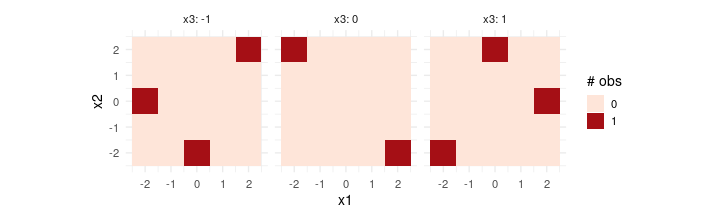
## verify correlations
design$corr(ortho_design) |> round(3)
#>         x1 x2 x3 I(x1^2) I(x2^2) I(x3^2)  x1:x2  x1:x3  x2:x3
#> x1       1  0  0   0.000   0.000   0.000  0.000  0.000  0.000
#> x2       0  1  0   0.000   0.000   0.000  0.000  0.000  0.000
#> x3       0  0  1   0.000   0.000   0.000  0.000  0.000  0.000
#> I(x1^2)  0  0  0   1.000  -0.333  -0.333  0.000  0.000 -0.816
#> I(x2^2)  0  0  0  -0.333   1.000  -0.333  0.000 -0.816  0.000
#> I(x3^2)  0  0  0  -0.333  -0.333   1.000  0.816  0.000  0.000
#> x1:x2    0  0  0   0.000   0.000   0.816  1.000 -0.500 -0.500
#> x1:x3    0  0  0   0.000  -0.816   0.000 -0.500  1.000  0.500
#> x2:x3    0  0  0  -0.816   0.000   0.000 -0.500  0.500  1.000

Higher-dimensional orthogonal designs

The "orthogonal" rounded design above belongs to the class of Orthogonal Minimally Aliased Response Surface (OMARS) designs introduced by (Núñez Ares and Goos 2020). As a higher-dimensional example, we construct a standard OMARS design (cf. (Núñez Ares and Goos 2020)) for a full quadratic model with 6 symmetric three-level factors x1 to x6. As orthogonality constraints, the main effects columns are required to be orthogonal with respect to all other design columns, similar to the previous example. In addition, the average level of each factor is zero, and the number of zeros in all main effects columns are equal ( $n_0^{ME}$ ) and the same for the number of zeros in all interaction columns ( $n_0^{IE}$ ).

data <- expand.grid(
  x1 = -1:1,
  x2 = -1:1,
  x3 = -1:1,
  x4 = -1:1,
  x5 = -1:1,
  x6 = -1:1
)

## initialize design object
design <- lm_design$new(
  formula = ~0 + (x1 + x2 + x3 + x4 + x5 + x6)^2 + I(x1^2) + I(x2^2) + I(x3^2) + I(x4^2) + I(x5^2) + I(x6^2),
  data = data,
  orthogonal = x1 + x2 + x3 + x4 + x5 + x6 ~ . ~ 0,
  zeros = list(
    ~ (x1 + x2 + x3 + x4 + x5 + x6)^2,
    ~ x1 + x2 + x3 + x4 + x5 + x6 + I(x1^2) + I(x2^2) + I(x3^2) + I(x4^2) + I(x5^2) + I(x6^2)
  ),
  col_means = x1 + x2 + x3 + x4 + x5 + x6 ~ 0
)

## exact omars design
(omars_design1 <- design$round(m = 16, method = "orthogonal", highs_control = list(log_to_console = FALSE)))
#>   [1] 0 0 0 0 0 1 0 0 0 0 0 0 0 0 0 0 0 0 0 0 0 0 0 0 0 0 0 0 0 0 0 0 0 1 0 0 0 0 0 0 0 0 0 0 0 0 0 0 0 0 0 0 0 0 0 0 0 0 0 0 0 0 0 0 0 0 0 0 0 0 0 0
#>  [73] 0 1 0 0 0 0 0 0 0 0 0 0 0 0 0 0 0 0 0 0 0 0 0 0 0 0 0 1 0 0 0 0 0 0 0 0 0 0 0 0 0 0 0 0 0 0 0 0 0 0 0 0 0 0 0 0 0 0 0 0 0 0 0 0 0 0 0 0 0 0 0 0
#> [145] 0 0 0 0 0 0 0 0 0 0 0 0 0 0 0 0 0 0 0 0 0 0 0 0 0 0 0 0 0 0 0 0 0 0 0 0 0 0 0 0 0 0 0 0 1 0 0 0 0 0 0 0 0 0 0 0 0 0 0 0 0 0 0 0 0 0 0 0 0 0 0 0
#> [217] 0 0 1 0 0 0 0 0 0 0 0 0 0 0 0 1 0 0 0 0 0 0 0 0 0 0 0 0 0 0 0 0 0 0 0 0 0 0 0 0 0 0 0 0 0 0 0 0 0 0 0 0 0 0 0 0 0 0 0 0 0 0 0 0 0 0 0 0 0 0 0 0
#> [289] 0 0 0 0 0 0 0 0 0 0 0 0 0 0 0 0 0 0 0 0 0 0 0 0 0 0 0 0 0 0 0 0 0 0 0 1 0 0 0 0 0 0 0 0 0 0 0 0 0 0 0 0 0 0 0 0 0 0 0 0 0 0 0 0 0 0 0 0 0 0 0 0
#> [361] 0 0 0 0 0 0 0 0 0 0 0 0 0 0 0 0 0 0 0 0 0 0 0 0 0 0 0 0 0 0 0 0 0 0 0 0 0 0 0 0 0 0 0 0 0 1 0 0 0 0 0 0 0 0 0 0 0 0 0 0 0 0 0 0 0 0 0 0 0 0 0 0
#> [433] 0 0 0 0 0 0 0 0 0 0 0 0 0 0 0 0 0 0 0 0 0 0 0 0 0 0 0 0 0 0 0 0 0 0 0 0 0 0 0 0 0 0 0 0 0 0 0 0 0 0 0 0 0 0 0 0 0 0 0 0 0 0 0 0 0 1 0 0 0 0 0 0
#> [505] 0 0 0 0 0 0 1 0 0 0 0 0 0 0 0 0 0 0 0 0 0 0 0 0 0 0 0 0 0 0 0 0 0 0 0 0 1 0 0 0 0 0 0 0 0 0 0 0 0 0 0 0 0 0 0 0 0 0 0 0 0 0 0 0 0 0 0 0 0 0 0 0
#> [577] 0 0 0 0 0 0 0 0 0 0 0 0 0 0 0 0 0 0 0 0 0 0 0 0 0 0 0 0 0 0 0 0 0 0 0 0 0 0 0 0 0 0 0 0 0 0 0 0 0 0 0 0 0 1 0 0 0 0 0 0 0 0 0 0 0 0 0 0 0 0 0 0
#> [649] 0 0 0 0 0 0 0 1 0 0 0 0 0 0 0 0 0 0 0 0 0 0 0 0 0 0 0 0 0 0 0 0 0 0 0 0 0 0 0 0 0 0 0 0 0 0 0 1 0 0 0 0 0 0 0 0 0 0 0 0 0 0 0 0 0 0 0 0 0 0 0 0
#> [721] 0 0 0 1 0 0 0 0 0
#> attr(,"criterion")
#> attr(,"criterion")$crit
#> [1] "alias"
#> 
#> attr(,"criterion")$crit.value
#> [1] 0.8743153
#> 
#> attr(,"criterion")$crit.rel.eff
#> [1] NA

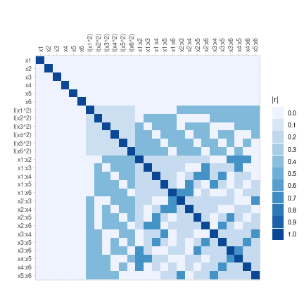
Besides the orthogonal argument, two other new arguments are used above: zeros and col_means.

The zeros argument allows to specify the proportion of zeros for sets of design columns in the form of one or more two-part formulas (e.g. ~ x1 + x2 + x3 + x4 + x5 + x6 ~ 0.125), included as extra (linear) equality constraints when optimizing the design. The left-hand side of each formula defines a set of design columns using linear model notation. The right-hand side specifies the proportion of zeros for the given set of design columns. If a one-part formula is provided as above, the proportion of zeros for each of the selected design columns is constrained to be the same, but no exact proportion is imposed. For exact designs, the zeros argument is only taken into account when using the "orthogonal" rounding method, in which case the proportions are converted to an exact number of zeros based on the requested design size $m$ .

The col_means argument constrains the designs column averages for sets of design columns. Similar to the orthogonal and zeros arguments, col_means accepts one or more two-part formulas (x1 + x2 + x3 + x4 + x5 + x6 ~ 0). The left-hand side of each formula selects the design columns and the right-hand side the requested column average subject to the optimized design. For exact designs, the col_means argument is only taken into account when the "orthogonal" rounding method is used.

Computational effort

As the number of columns $p$ in the design matrix $\boldsymbol{X}$ grows, it becomes computationally more expensive (i.e. more time-consuming) to solve the MILP and find a valid orthogonally constrained design. As of HiGHS version 1.15.0, the MILP can be solved in parallel using multiple CPU cores to reduce the runtime. Another option is to export the MILP as a generic MPS file using the highs_write_mps argument when calling $round(). This allows to solve the MILP using an external (commercial) solver, e.g. CPLEX, Gurobi, Mosek, or if a GPU is available, using the open-source cuOpt solver.

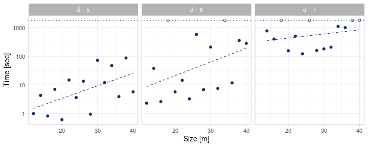
The figure below highlights observed computation times (in seconds) to solve for exact OMARS designs of different sizes $m$ . From left to right, the model corresponds to a $d$ -factor full quadratic model, with $2d + d(d-1)/2$ design columns and design grid of size $3^d$ . The figure displays the computation times for the HiGHS MILP solver (v1.15.1) to find a single feasible solution (mip_max_improving_sols = 1L) using a single core on a modern laptop computer (Intel i7-8550U CPU). The maximum runtime was set to 1800 seconds, the design configurations that did not find any feasible solution within this time limit are highlighted by open circles.

References

Cederberg, D., and S. Boyd. 2025. “Projections onto Spectral Matrix Cones.” arXiv Preprint arXiv:2511.01089.

Fedorov, V. V. 1972. Theory of Optimal Experiments. Academic Press.

Núñez Ares, J., and P. Goos. 2020. “Enumeration and Multicriteria Selection of Orthogonal Minimally Aliased Response Surface Designs.” Technometrics 62 (1): 21–36.

Pukelsheim, F., and S. Rieder. 1992. “Efficient Rounding of Approximate Designs.” Biometrika 79 (4): 763–70.

Sagnol, G., and R. Harman. 2015. “Computing Exact D-Optimal Designs by Mixed Integer Second-Order Cone Programming.” The Annals of Statistics 43 (5): 2198–224. https://doi.org/10.1214/15-AOS1339.