Example gallery

Optimization

Volcano height dataset

The volcano dataset included in the datasets R-package reports topographic information of the Maunga Whau (Mt Eden) volcano in the Auckland volcano field. To reduce the data grid size, we first downsample the volcano data, resulting in volcano heights across a $(44 \times 31)$-dimensional matrix with rows corresponding to grid lines running east to west and columns to grid lines running south to north.

## initialize data
data(volcano)

## subsample grid
volcano <- volcano[c(TRUE, FALSE), c(TRUE, FALSE)]

data <- expand.grid(
  x1 = seq(from = -1, to = 1, length = dim(volcano)[1]),
  x2 = seq(from = -1, to = 1, length = dim(volcano)[2])
)
## standardize response
data[["y"]] <- (c(volcano) - min(volcano)) / (max(volcano) - min(volcano))

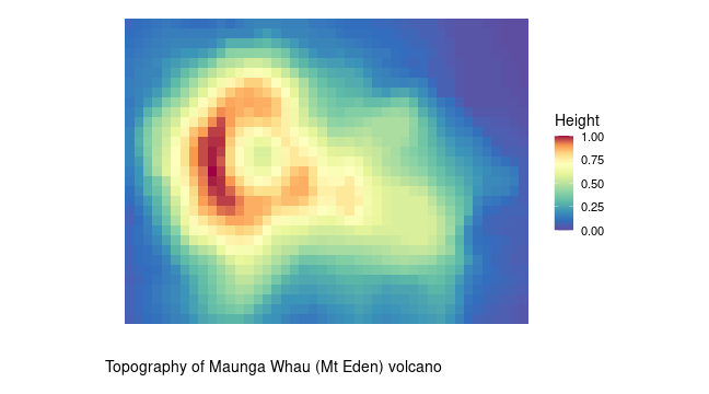
The irregular height response surface is not easily captured by a parametric linear or nonlinear model. Instead, a nonparametric regression model, such as a generalized additive model (GAM) or a Gaussian process regression (GPR) model, is better suited, allowing the complexity of the model to grow with the number of observations. In vignette("glm_gam_design"), the use of a GAM to model the volcano height was already discussed. In this example, we consider penalized design augmentation subject to a GPR prediction model, which is expected to behave similar to (multi-proposal) Bayesian Optimization. The objective is to maximize the observed height response, where the observed height at a specific grid point is assumed to be noise-free.

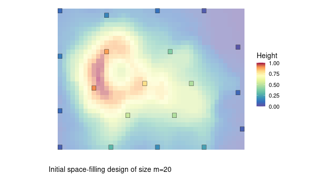
As an initial design, a space-filling design of size $m = 20$ is generated using the distance-based "dist-min" rounding method:

library(cvxoptdes)

## initial design
design <- lm_design$new(
  formula = ~ x1 + x2,
  data = data
)

init_design <- design$round(m = 20, method = "dist-min", seed = 1, max_iter = 200, design_weights = FALSE)

Given the observed data, a Gaussian process model with RBF kernel is fitted using HMC sampling in Stan (see e.g. https://mc-stan.org/docs/stan-users-guide/gaussian-processes.html), according to:

The GP model has three kernel parameters to estimate: the marginal standard deviation ($\sigma$) of the kernel and two length-scale parameters ($\rho = (\rho_1, \rho_2)$), one for each dimension. The responses are assumed to be noise-free, for this reason only a small constant $\lambda = 1e-8$ is added to the diagonal of the GP kernel/covariance matrix to ensure positive definiteness.

The section Gaussian process regression in vignette("augment_design") explains how the GP model can be expressed as an (approximate) Bayesian linear model with design matrix $\Phi$ depending on the estimated kernel $k(\boldsymbol{x}, \boldsymbol{z})$. Using the posterior medians of the kernel parameters ($\sigma$, $\rho$), the $(n \times m)$-dimensional $\Phi$ matrix is calculated by stacking row vectors:

where $L_{XX}^{-1}$ is the inverse of the Cholesky square root of $K_{XX} \in \mathbb{R}^{p \times p}$ and $k(\boldsymbol{X}, \boldsymbol{x}_i)$ is the cross-kernel vector between $\boldsymbol{X}$ and $\boldsymbol{x}_i$ with elements $k(\boldsymbol{x}_j, \boldsymbol{x}_i)$. Note that the $(m \times m)$-submatrix of $\Phi$ with rows corresponding to the design points in $\boldsymbol{X}$ is exactly the square root ($L_{XX}$) of $K_{XX}$.

The design can now be augmented in exactly the same way as for a linear model with $(n \times m)$ design matrix $\Phi$ and a small ridge penalty $\lambda = 1e-8$ to regularize the information matrix. To balance optimization of the design criterion (exploration) and maximization of the response (exploitation), we include costs proportional to (one minus) the GP posterior mean thereby giving preference to design points with a higher predicted response.

## for demonstration only
Phi <- { ... }          ## GP linear model design matrix         (n x m)
mu <- { ... }           ## GP posterior mean across design space (n x 1)

design <- lm_design$new(
  formula = ~ 0 + .,    ## linear model
  data = Phi,           
  lambda = 1e-8,        ## ridge penalty
  alpha = 0.05,         ## cost scaling
  cost = 1 - mu         ## exploitation costs
)

## approximate I-optimal augmented design
design$augment(design_weights = init_design, criterion = "I", return_value = FALSE)

## exact I-optimal design augmentation w/ 5 design points
design$round(m = 5, method = "optimal", augment_design = init_design, replicates = FALSE)

This approach can be iterated multiple times analogous to standard Bayesian Optimization, where in each iteration the GP model is refitted and the design matrix $\Phi$ and cost values $\mu$ are updated accordingly.

In the first figure below, 8 design augmentation iterations are performed using a zero cost penalty ($\alpha = 0$) starting from the initial design of size $m = 20$, and adding 5 new design points in each iteration. This means that the only target in the design augmentation is optimization of the I-criterion, i.e. minimizing the average GP prediction variance across the design grid, which corresponds to pure exploration. For each iteration, the current MSE and $R^2$ of the GP predictions (across the full design space) and the current highest observed response are displayed. The plotted response surfaces are the predicted surfaces based on the available GP (posterior mean) predictions. The second figure displays the results of the same sequential design augmentation procedure, but with a small non-zero cost penalty ($\alpha = 0.05$), meaning that the design is augmented by penalizing the I-criterion based on the current GP predictions.

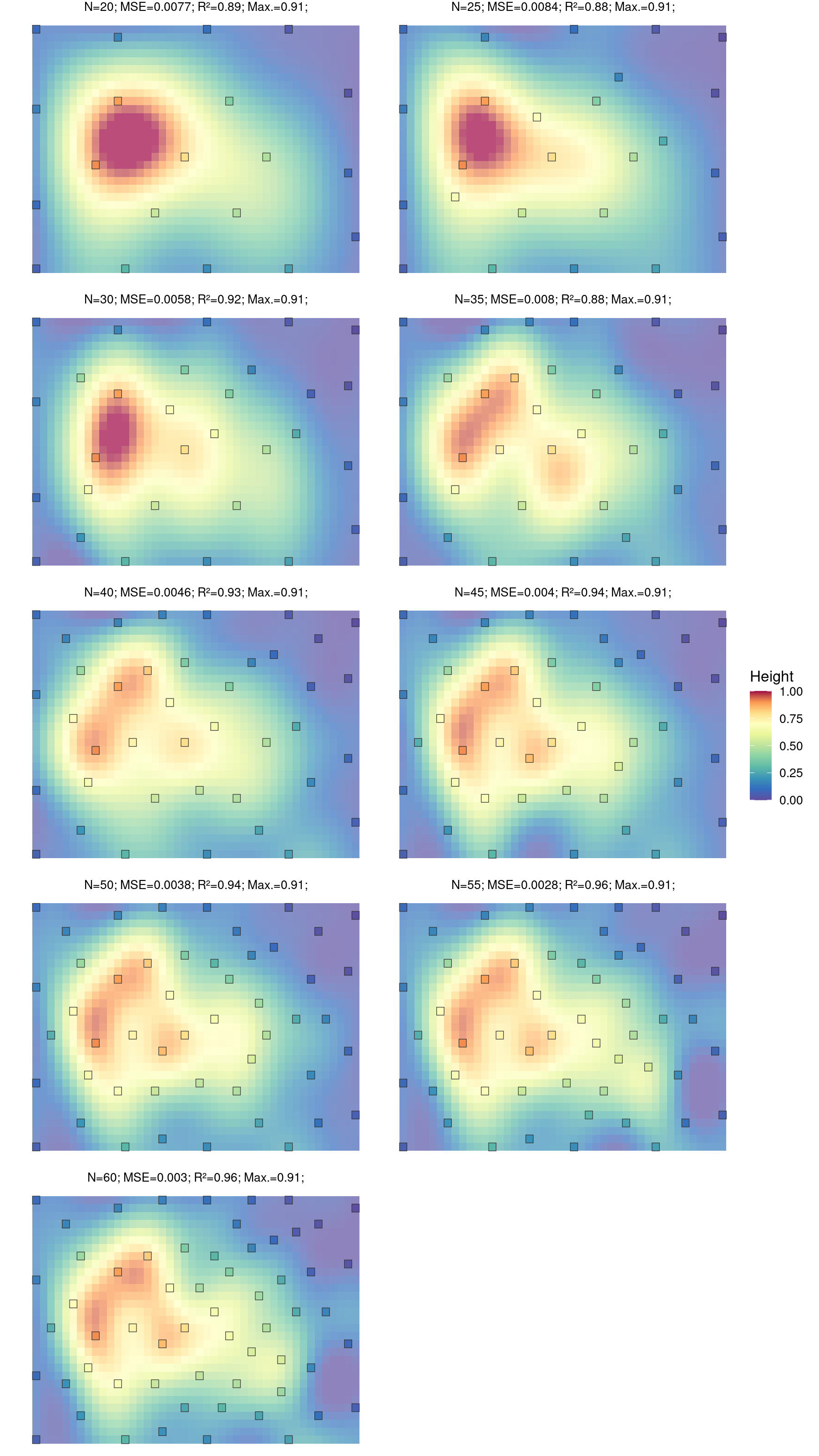
I-optimal design augmentation (pure exploration)

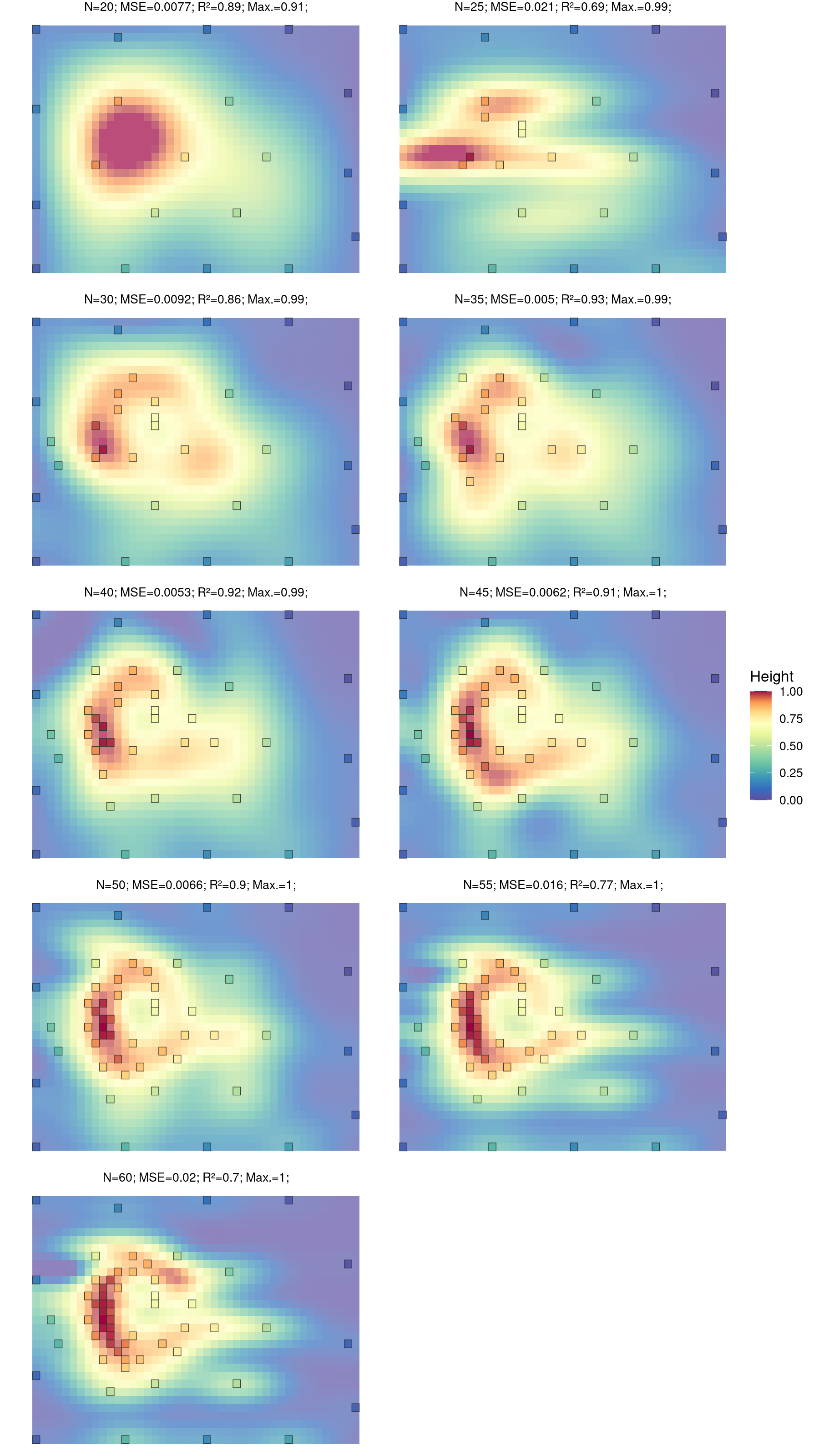
Penalized I-optimal design augmentation α=0.05 (exploration/exploitation)

Caco-2 (cell effective permeability)

This dataset from (Wang 2016) reports the Caco-2 cell effective permeability given 906 drug SMILES strings and is publicly available at https://tdcommons.ai/single_pred_tasks/adme/#caco-2-cell-effective-permeability-wang-et-al. The objective is to evaluate the drug compounds maximizing the permeability response. In a first step, a continuous vector of molecular descriptors (947 features) is generated for each drug compound using fastprop. The initial descriptor vectors are reduced to vectors of size 106 using kernel PCA (standard RBF kernel) explaining 99% of the variation in the original set of molecular descriptors.

The figure visualizes the molecular descriptors (106 features) using a t-SNE projection to 2D space, where the response has been standardized to the unit interval.

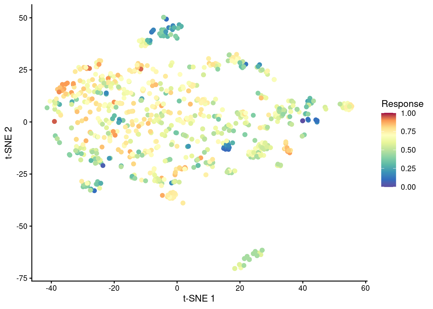
Molecular descriptors in 2D space

Assuming no prior knowledge of the target responses, we consider a sequential design approach based on a simple linear model containing a single (main effects) term for each feature. No interactions are taken into account to minimize the number of model parameters to be estimated. All designs of size smaller than 106 result in a singular information matrix. For this reason, we include a small ridge penalty $\lambda = 10^{-4}$, which is added to the diagonal of the information matrix to ensure positive definiteness also for smaller design sizes. The initial design is a (regularized) D-optimal design of size $n_0 = 50$, and we augment the design by 25 new design points a total of 10 times. In each iteration, costs are updated using (the inverse of) the predicted permeability responses obtained by performing a lasso regression on the available data with glmnet. The lasso penalty is selected using 10-fold cross-validation.

## main effects model
frm <- sprintf("~ %s", paste(sprintf("%s", names(features)), collapse = " + "))
design <- lm_design$new(
  formula = as.formula(frm),
  data = features,
  lambda = 1e-4,     ## ridge penalty
  alpha = 0.5        ## cost penalty
)

## initial D-optimal design
design$optimize(criterion = "D", scs_control = list(time_limit_secs = 60), return_value = FALSE)
init_design <- design$round(m = 50, method = "optimal", seed = 1)
new_design <- init_design

for(iter in 1:10) {
  ## update cost function
  fit <- cv.glmnet(x = features[new_design > 0], y = y[new_design > 0], nfolds = 10)
  design$update(cost = 1 / predict(fit, newx = features, s = "lambda.min"))
  ## augment D-optimal design
  design$augment(design_weights = new_design, criterion = "D", return_value = FALSE)
  new_design <- design$round(m = 25, method = "optimal", seed = 1, replicates = FALSE, augment_design = new_design)
}

The first figure below displays the selected design points after the initial design of size $n_0 = 50$ up to the final design of size $n = 300$ using a zero cost penalty ($\alpha = 0$), meaning that the design is augmented only in terms of the (regularized) D-criterion (i.e. pure exploration). For each iteration, the current MSE and $R^2$ (for all responses) of the lasso predictions and the current highest observed response and the percentage of observations sampled from the upper 10% response values are displayed.

The second figure displays the selected design points after the initial design of size $n_0 = 50$ up to the final design of size $n = 300$ using a non-zero cost penalty ($\alpha = 0.5$), meaning that the design is augmented by penalizing the (regularized) D-criterion based on the current lasso predictions (i.e. exploration/exploitation trade-off).

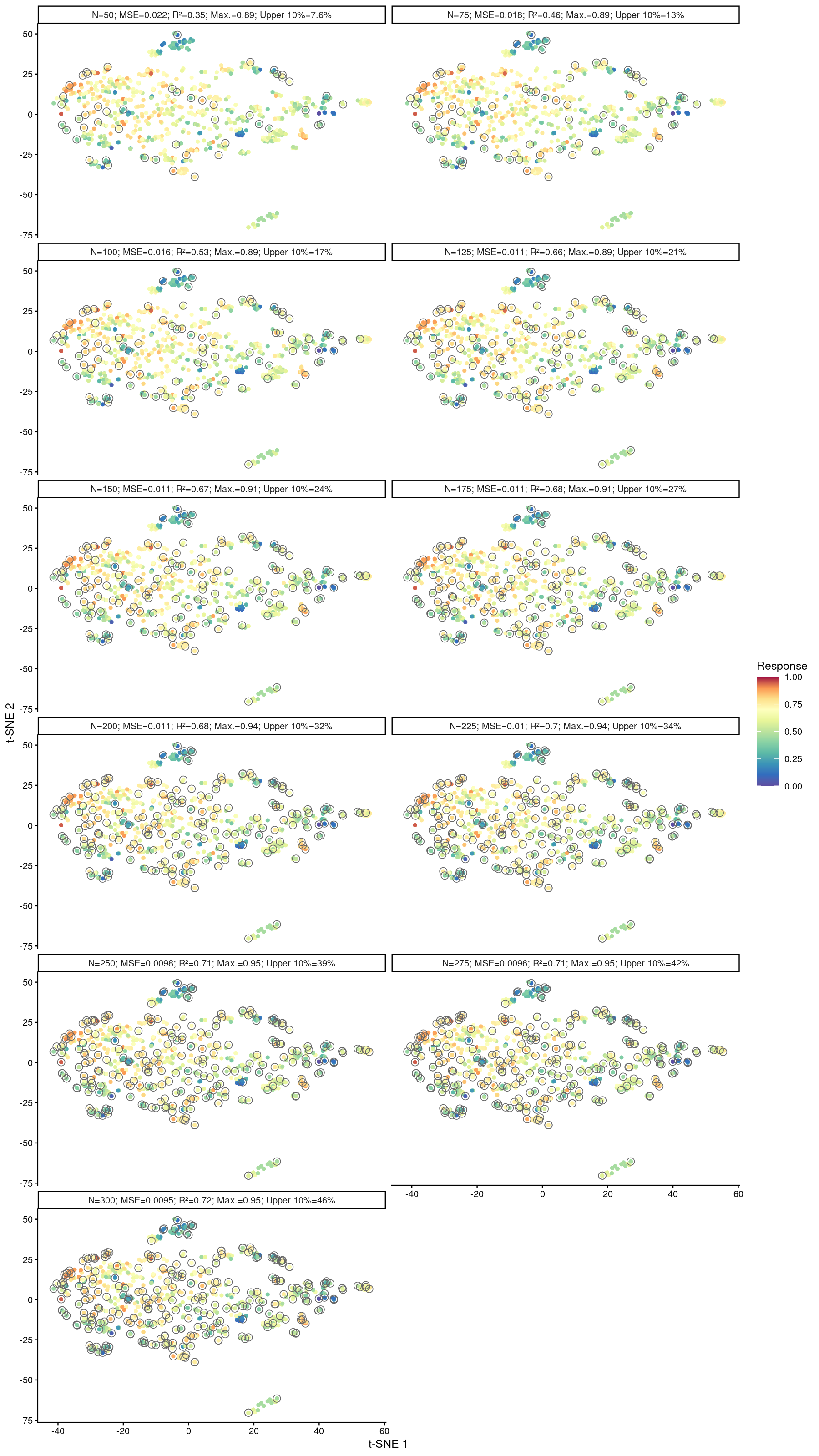
D-optimal design augmentation (pure exploration)

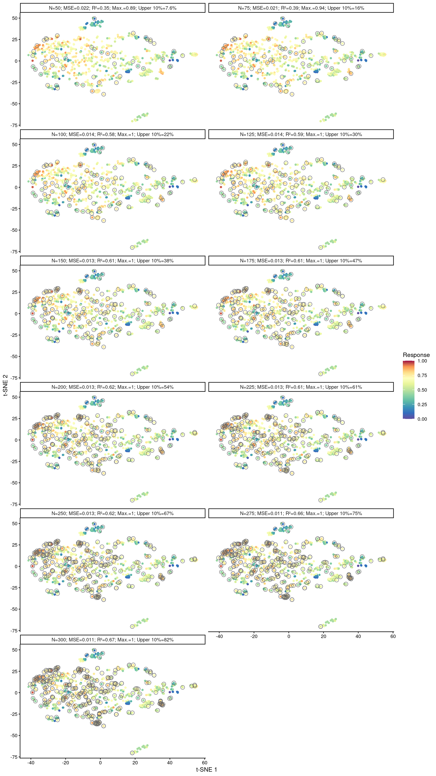
Penalized D-optimal design augmentation α=0.5 (exploration/exploitation)

SARS-CoV-2 drug activity

This dataset consists of binary levels of activity against SARS-CoV-2 3CL Protease for 880 drug compounds identified by their SMILES strings, (78 high- versus 802 low-activity compounds). The high-throughput screening data was reported by Diamond Light Source and is publicly available at https://tdcommons.ai/single_pred_tasks/hts/#sars-cov-2-3cl-protease-diamond. Viewing this as a drug discovery problem, our aim is to efficiently identify a maximum number of drug compounds with a high activity response, assuming nu initial knowledge of the activity responses.

To initialize the candidate design grid, binary (1024-bit) Morgan fingerprints are generated for each drug molecule from their SMILES strings using RDKit. The visualization shows a t-SNE projection of the high-dimensional molecular descriptors to 2D space, which manages to cluster a set of high-activity compounds using two T-SNE components:

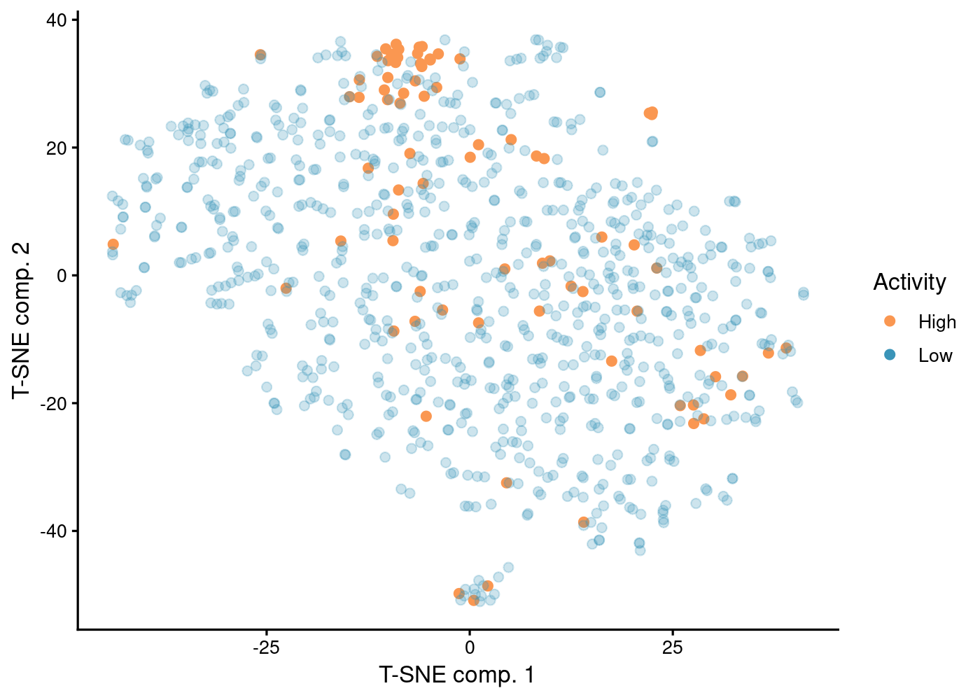
Molecular fingerprints in 2D space

The initial design is a regularized D-optimal design for a linear model including only the fingerprint main effects ($p = 1024$) of size $m = 50$ using a small ridge penalty $\lambda = 10^{-2}$ to regularize the information matrix. After evaluation of the initial design, a Gaussian process logistic regression model is fitted to the available data according to:

The projection vector $\phi_X(\boldsymbol{x}_i)^T$, as given in vignette("augment_design"), is defined using a parameterized Tanimoto (or Jaccard) kernel to measure similarity between binary fingerprints:

The kernel is parameterized by a magnitude $\sigma$ and a length-scale $\rho$, which are estimated together with the latent coefficient vector $\boldsymbol{\theta}$ when fitting the logistic regression model. Given the estimated projection matrix $\widehat{\Phi}(\mathcal{X}, \boldsymbol{X}) \in \mathbb{R}^{n \times m}$ and the predicted probabilities $\hat{p}(\boldsymbol{x})$ over the candidate design grid, a new glm_design object is initialized with design matrix $\widehat{\Phi}(\mathcal{X}, \boldsymbol{X})$ and nominal parameter values $\hat{\boldsymbol{\theta}}$ as:

## for demonstration only
Phi <- { ... }                                ## fitted GP projection matrix         (n x m)
theta <- { ... }                              ## fitted coefficients                 (m x 1)
p <- 1 / (1 + exp(-(Phi %*% theta)))          ## predicted probabilities             (n x 1)

design <- glm_design$new(
  formula = ~ 0 + .,
  data = Phi,
  family = binomial(link = "log"),
  theta = theta,
  cost = 1 - p
)

design$augment(design_weights = current_design, criterion = "D", return_value = FALSE)
design$round(m = 50, method = "optimal", seed = 1, replicates = FALSE, n_repeats = 50, augment_design = current_design)

The new design object imposes additive cost penalties $c(\boldsymbol{x}) = 1 - \hat{p}(\boldsymbol{x})$, penalizing compounds with a low predicted activity. The global penalty scaling parameter is kept at the default $\alpha = 1$. With the new design object, the existing design is augmented by $m_1 = 50$ new compounds using D-optimality as the optimization criterion. The figure displays the percentage of identified high-activity compounds by augmenting the design 5 times with 50 compounds, updating the data, theta and cost arguments in the glm_design object after each iteration. The open circles highlight the compounds included in the sequentially augmented design in the t-SNE projected 2D space, showing the strong bias towards the cluster of high-activity compounds. In general, the performance of the demonstrated online design approach depends heavily on the accuracy of the model predictions. In this example, identifying the complete set of high-activity compounds becomes increasingly hard due to the inability of the model to correctly predict the response of the unobserved high-activity compounds using only the binary molecular fingerprints. The Gaussian process logistic regression model was fitted in Stan by optimizing the maximum a posteriori (MAP) estimates of the parameters.

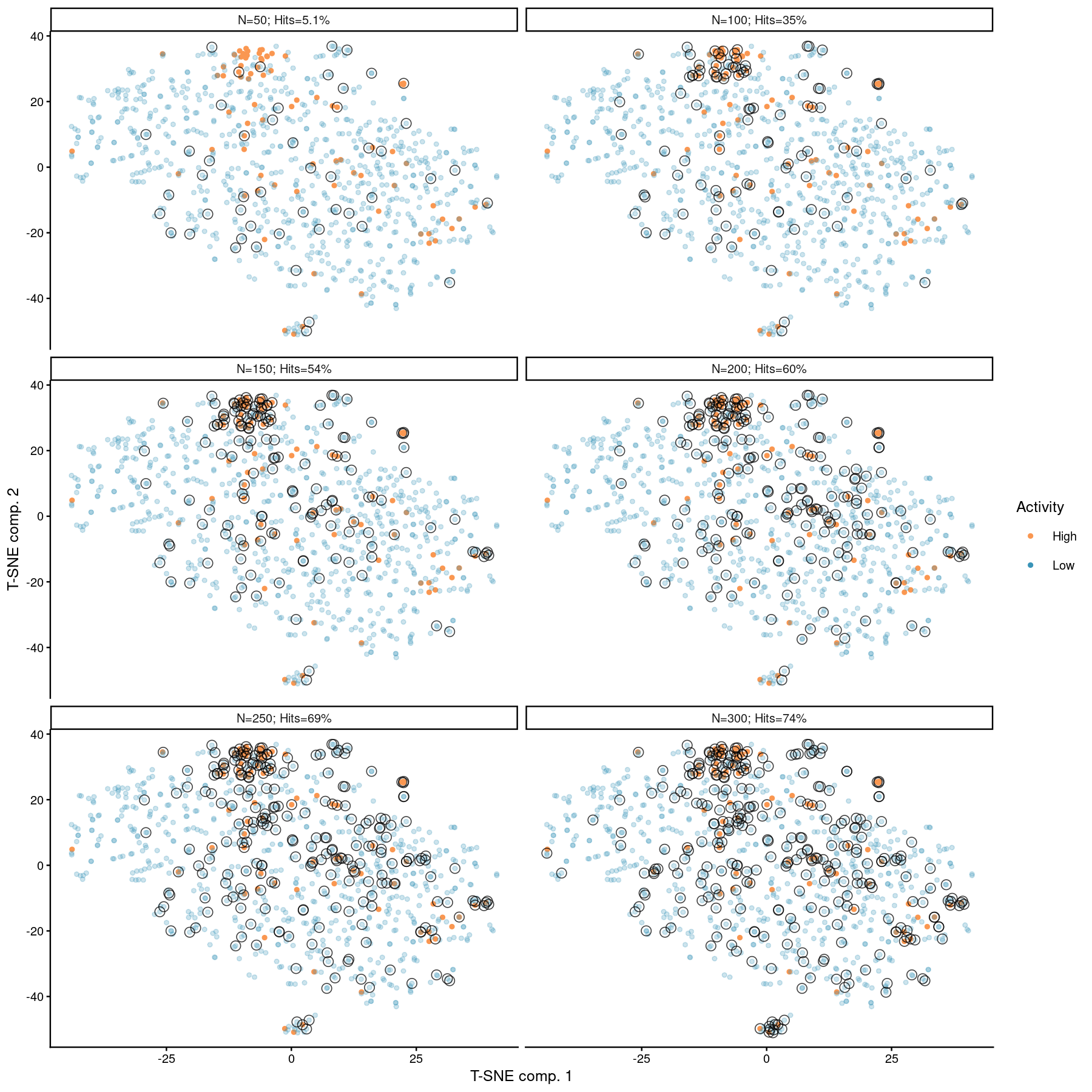
Penalized D-optimal design augmentation (5 times 50 compounds)

References

Wang, N. et al. 2016. “ADME Properties Evaluation in Drug Discovery: Prediction of Caco-2 Cell Permeability Using a Combination of NSGA-II and Boosting.” Journal of Chemical Information and Modeling 56 (4): 763–73.